Works

The polar equation r = a cos(kθ) draws a rose, and an integer k sets how many petals appear.

The curve x = A sin(at + δ), y = B sin(bt) takes its shape from the frequency ratio a:b and the phase δ.

A damped harmonograph traces x = A sin(at + δ) e^(-dt), y = B sin(bt) e^(-dt), and frequency, phase, and damping set how the orbit closes in.

A hypotrochoid is the path of a pen on a circle rolling inside a fixed circle; R and r set the corners, and d sets how sharp they are.

Two opposite traveling waves of equal amplitude and frequency add to y = 2A sin(kx) cos(ωt), whose nodes and antinodes stay fixed.

Two sources draw the curves where the path difference is an integer multiple of the wavelength.

Points on a square gather where the amplitude of the selected mode is zero.

Bars and equal-height rectangles show arithmetic and geometric sequences and the formulas for their sums.

Quarter-circles on squares of Fibonacci side lengths approximate a logarithmic spiral.

Rays from the focus reflect off the parabola and leave parallel to its axis.

Partial sums, stacked areas, and a sine product picture the sum of reciprocal squares, equal to pi squared over 6.

A family of lines sliding on the two axes weaves a parabolic envelope in all four quadrants.

Period doubling and chaotic regions of x_{n+1} = r x_n(1-x_n) as the parameter r changes.

A self-similar triangle fractal, made by recursively removing the middle triangle or by the chaos game.

A point travels on an ellipse, with a segment drawn from it to each focus.

A 2×2 matrix acts on the plane grid, and the figure shows shear together with vertical scaling.

Affine maps that combine translation, rotation, and scaling, iterated on a pattern.

The matrix product of repeated rotation and uniform scaling, and the spirals and logarithmic spirals it generates.

An iterated function system (IFS) iterates several affine maps and generates a self-similar fractal.

Rectangles approach the area under a curve, and the sum settles as the number of partitions grows.

The secant slope approaches the tangent slope, so the derivative reads as an instantaneous rate of change.

A rope of fixed length tows a point along a tractrix, with sech and tanh and a symmetric pair of tracks.

The radius r = a e^(bθ) grows with the angle, and every ray from the origin meets the curve at one fixed angle.

Paths found by integrating along a vector field, a geometric picture of the solutions of a differential equation.

Two rotating phasors join head to tail, and their sum traces how harmonic waves superpose as amplitude, frequency ratio, and phase difference change.

On the complex plane, addition combines vectors, and multiplication scales by the moduli and rotates by the sum of the arguments.

Any nonzero complex number is written as z = re^(iθ), with modulus r and argument θ, linking rectangular and polar coordinates.

Euler's formula e^(iθ) = cos θ + i sin θ rotates a vector on the complex plane and traces the sine wave of its imaginary part.

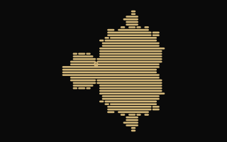
Iterating z to z squared plus c on the complex plane draws a fractal boundary and its self-similar structure.

A triangular array of binomial coefficients, showing the recurrence, the symmetry, and combinatorial identities.

With only right and up steps, the number of paths from the origin to (m, n) is C(m+n, m).

Cutting a square or a cube into blocks shows the expansion of (a+b)^n and where its coefficients come from.

Catalan numbers count matched parentheses, lattice paths that do not cross the diagonal, and triangulations of a convex polygon.

Tree diagrams and area ratios show what P(A|B) means, and how Bayes' theorem updates it.

The histogram of successes in n trials moves toward a bell-shaped normal curve as n grows.

Drop needles at random and estimate π from how often a needle crosses a line.

Exponential growth and decay of y = Ce^(kt), with doubling time, half-life, and slope proportional to height.

A logarithmic scale turns equal ratios into equal steps, so exponential growth becomes a straight line.

Define ln t as the integral of 1/x from 1 to t, and e as the unique positive number with ln e = 1.

The logistic curve y = L/(1+a e^(-kt)) rises, then levels off at the carrying capacity L.

Add two plane vectors by the parallelogram rule, and scale one of them, to see how a linear combination is built.

The dot product, or inner product, reads the angle between two vectors, a right angle, and the work of a force.

Split a vector into a part along a chosen direction and a part at right angles to it, and drag to see the length change with the angle.

Sources, sinks, vortices, and saddles, the typical vector fields that give a geometric vocabulary for direction fields.

Drag the angle θ on the unit circle and read cos θ, sin θ, tan θ, and the sign in each quadrant.

Drag the vertices of a triangle, switch between the sine law and the cosine law, and check the side-angle relations and the circumradius.

Drag α and β on the unit circle and read the sum-to-product identities through the midpoint angle m and the offset d.

Drag a point on the graph and watch (a, b) reflect across y = x to (b, a) on the inverse.

Drag the zeros and set each multiplicity to 1 or 2, and watch the graph cross or touch the x-axis.

Drag a, b, and c to compare the general form with the vertex form, and watch the vertex, the axis, and the x-intercepts follow the discriminant.

Drag a, b, h, and k to see how y = a f(b(x - h)) + k shifts, stretches, and flips a basic graph.

Drag the angle θ on the circle and read the arc length s together with the radian measure θ = s/r.

Drag A, T, φ, and k to compare y = A sin(2π(x-φ)/T) + k with the base sine wave.

Switch among standard 2×2 matrices and see that an eigenvector's line still maps to itself, with the stretch set by the eigenvalue.

Change the degree n and the center a, and watch the Taylor polynomial fit sin x, cos x, and e^x locally.

Compare f(x) with f'(x), and watch increase, extrema, and the tangent slope move together.

Move a zero and the asymptotes, and watch the graph blow up at an uncancelled denominator zero and level off far away.

Move the slope and the intercept, and watch the quotient line and the remainder set the far trend.

Drag points in a two-dimensional cloud and watch the direction, the correlation r, and the least-squares line change together.

Keep the main cloud fixed and move one highlighted point to see how its horizontal distance and residual pull the least-squares line.

Sort one-dimensional values and drag them to watch the median, the interquartile range, and the tail outliers update.

Switch the binomial B(n, p) and the geometric Geo(p), and drag p to compare the bars with E(X) and Var(X).

Change the angle, length, and tilt of two spatial vectors and read the parallelogram area, the normal n, and the angle together.

Drag the components and watch the projections on the xy, xz, and yz planes describe one vector in space.

Drag the start and direction of a line, and the normal and constant of a plane, and watch an intersection, a parallel line, or a line lying in the plane.

Drag the normal n and a point fixed on the plane, and read ax+by+cz=h together with the distance from a point to the plane.

Drag the constraint lines and watch how the half-plane masks and the convex feasible polygon change as they intersect.

Drag a level line of the objective z=px+qy and watch the whole plane split into layers by a family of parallel lines.

Visit each vertex of the feasible region, compute z=px+qy, and read from the candidate table where the optimal solution lies.

Drag a point in the plane and watch the gradient stay orthogonal to the level curve, pointing where the function increases fastest.

Drag a complex number z and watch a power multiply the argument by n, or roots divide the circle into n equal parts.

Pick c on the Mandelbrot set and the corner draws the corresponding Julia set.

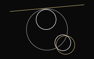
Invert a line and a circle in a fixed circle, and see whether each image is a circle or a line.

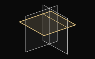
Three planes stand for a system of linear equations, and adding a multiple of the first row to the third turns that plane while the common solution stays put.

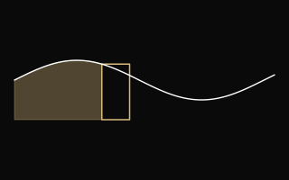
As h approaches 0, the area increment divided by the width approaches the height of the curve.

On the unit disk, an equilateral triangle whose sides are arcs orthogonal to the boundary has a smaller angle sum nearer the edge.

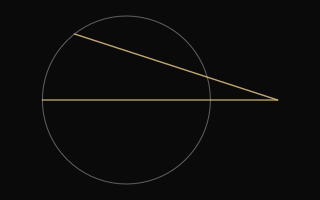
From one point outside a circle, each secant's external part times the whole secant is the same number.

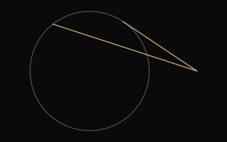
From a point outside a circle, the square of the tangent segment equals the secant's external part times the whole secant.